For published studies, this command calculates (1) how much bias there must be in an estimate to invalidate/sustain an inference; (2) the impact of an omitted variable necessary to invalidate/sustain an inference for a regression coefficient.
pkonfound(
  est_eff,
  std_err,
  n_obs,
  n_covariates = 1,
  alpha = 0.05,
  tails = 2,
  index = "RIR",
  nu = 0,
  n_treat = NULL,
  switch_trm = TRUE,
  model_type = "ols",
  a = NULL,
  b = NULL,
  c = NULL,
  d = NULL,
  two_by_two_table = NULL,
  test = "fisher",
  replace = "control",
  sdx,
  sdy,
  R2,
  eff_thr = 0,
  FR2max,
  FR2max_multiplier = 1.3,
  to_return = "print"
)
Arguments
- est_eff
the estimated effect (such as an unstandardized beta coefficient or a group mean difference)
- std_err
the standard error of the estimate of the unstandardized regression coefficient
- n_obs
the number of observations in the sample
- n_covariates
the number of covariates in the regression model
- alpha
probability of rejecting the null hypothesis (defaults to 0.05)
- tails
integer whether hypothesis testing is one-tailed (1) or two-tailed (2; defaults to 2)
- index
whether output is RIR or IT (impact threshold); defaults to "RIR"
- nu
what hypothesis to be tested; defaults to testing whether est_eff is significantly different from 0
- n_treat
the number of cases associated with the treatment condition; applicable only when model_type = "logistic"
- switch_trm
whether to switch the treatment and control cases; defaults to FALSE; applicable only when model_type = "logistic"
- model_type
the type of model being estimated; defaults to "ols" for a linear regression model; the other option is "logistic"
- a
cell is the number of cases in the control group showing unsuccessful results
- b
cell is the number of cases in the control group showing successful results
- c
cell is the number of cases in the treatment group showing unsuccessful results
- d
cell is the number of cases in the treatment group showing successful results
- two_by_two_table
table that is a matrix or can be coerced to one (data.frame, tibble, tribble) from which the a, b, c, and d arguments can be extracted
- test
whether using Fisher's Exact Test or A chi-square test; defaults to Fisher's Exact Test
- replace
whether using entire sample or the control group to calculate the base rate; default is the control group
- sdx
the standard deviation of X
- sdy
the standard deviation of Y
- R2
the unadjusted,original R2 in the observed function
- eff_thr
unstandardized coefficient threshold to change an inference
- FR2max
the largest R2, or R2max, in the final model with unobserved confounder
- FR2max_multiplier
the multiplier of R2 to get R2max, default is set to 1.3
- to_return
whether to return a data.frame (by specifying this argument to equal "raw_output" for use in other analyses) or a plot ("plot"); default is to print ("print") the output to the console; can specify a vector of output to return
Value
prints the bias and the number of cases that would have to be replaced with cases for which there is no effect to invalidate the inference
Examples
# using pkonfound for linear models
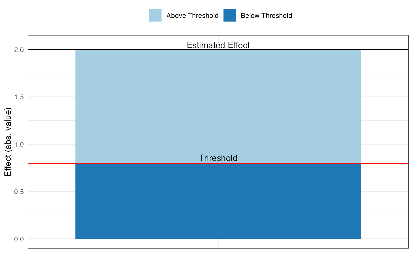
pkonfound(2, .4, 100, 3)
#> Robustness of Inference to Replacement (RIR):
#> To invalidate an inference, 60.29 % of the estimate would have to be due to bias.
#> This is based on a threshold of 0.794 for statistical significance (alpha = 0.05).
#>
#> To invalidate an inference, 60 observations would have to be replaced with cases
#> for which the effect is 0 (RIR = 60).
#>
#> See Frank et al. (2013) for a description of the method.
#>
#> Citation: Frank, K.A., Maroulis, S., Duong, M., and Kelcey, B. (2013).
#> What would it take to change an inference?
#> Using Rubin's causal model to interpret the robustness of causal inferences.
#> Education, Evaluation and Policy Analysis, 35 437-460.
#> For other forms of output, run ?pkonfound and inspect the to_return argument
#> For models fit in R, consider use of konfound().
pkonfound(-2.2, .65, 200, 3)
#> Robustness of Inference to Replacement (RIR):
#> To invalidate an inference, 41.728 % of the estimate would have to be due to bias.
#> This is based on a threshold of -1.282 for statistical significance (alpha = 0.05).
#>
#> To invalidate an inference, 83 observations would have to be replaced with cases
#> for which the effect is 0 (RIR = 83).
#>
#> See Frank et al. (2013) for a description of the method.
#>
#> Citation: Frank, K.A., Maroulis, S., Duong, M., and Kelcey, B. (2013).
#> What would it take to change an inference?
#> Using Rubin's causal model to interpret the robustness of causal inferences.
#> Education, Evaluation and Policy Analysis, 35 437-460.
#> For other forms of output, run ?pkonfound and inspect the to_return argument
#> For models fit in R, consider use of konfound().
pkonfound(.5, 3, 200, 3)
#> Robustness of Inference to Replacement (RIR):
#> To sustain an inference, 91.549 % of the estimate would have to be due to bias.
#> This is based on a threshold of 5.917 for statistical significance (alpha = 0.05).
#>
#> To sustain an inference, 183 of the cases with 0 effect would have to be replaced with cases at the threshold of inference (RIR = 183).
#> See Frank et al. (2013) for a description of the method.
#>
#> Citation: Frank, K.A., Maroulis, S., Duong, M., and Kelcey, B. (2013).
#> What would it take to change an inference?
#> Using Rubin's causal model to interpret the robustness of causal inferences.
#> Education, Evaluation and Policy Analysis, 35 437-460.
#> For other forms of output, run ?pkonfound and inspect the to_return argument
#> For models fit in R, consider use of konfound().
pkonfound(-0.2, 0.103, 20888, 3, n_treat = 17888, model_type = "logistic")
#> Conclusion:
#> User-entered Table:
#> Fail Success
#> Control 2882 118
#> Treatment 17308 580
#>
#> Note: Values have been rounded to the nearest integer.This may cause a little change to the estimated effect for the Implied Table.
#>
#> To sustain an inference for a negative treatment effect, you would need to replace 2 treatment success cases
#> with cases for which the probability of failure in the control group applies (RIR = 2).
#> This is equivalent to transferring 1 case from treatment success to treatment failure,
#> as shown, from the Implied Table to the Transfer Table.
#>
#> Transfer Table:
#> Fail Success
#> Control 2882 118
#> Treatment 17309 579
#>
#> For the Implied Table, we have an estimate of -0.200, with a SE of 0.103 and a t-ratio of -1.946.
#> For the Transfer Table, we have an estimate of -0.202, with a SE of 0.103 and a t-ratio of -1.963.
#>
#> RIR:
#> RIR = 2
#> For other forms of output, run ?pkonfound and inspect the to_return argument
#> For models fit in R, consider use of konfound().
pkonfound(2, .4, 100, 3, to_return = "thresh_plot")
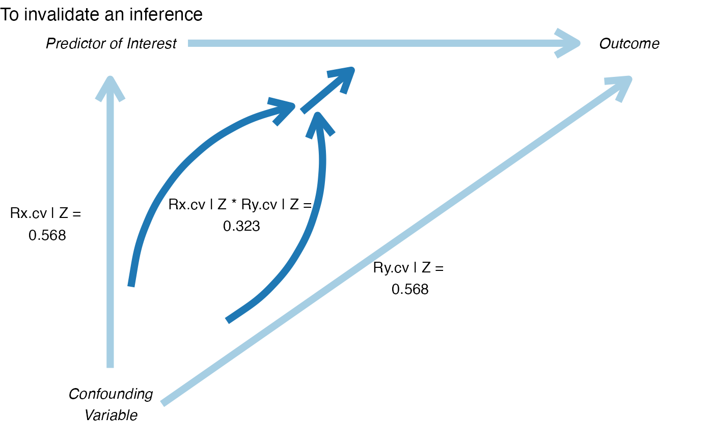
 pkonfound(2, .4, 100, 3, to_return = "corr_plot")
 pkonfound_output <- pkonfound(2, .4, 200, 3,
to_return = c("raw_output", "thresh_plot", "corr_plot")
)
#> Robustness of Inference to Replacement (RIR):
#> To invalidate an inference, 60.555 % of the estimate would have to be due to bias.
#> This is based on a threshold of 0.789 for statistical significance (alpha = 0.05).
#>
#> To invalidate an inference, 121 observations would have to be replaced with cases
#> for which the effect is 0 (RIR = 121).
#>
#> See Frank et al. (2013) for a description of the method.
#>
#> Citation: Frank, K.A., Maroulis, S., Duong, M., and Kelcey, B. (2013).
#> What would it take to change an inference?
#> Using Rubin's causal model to interpret the robustness of causal inferences.
#> Education, Evaluation and Policy Analysis, 35 437-460.
#>
#> Print output created by default. Created 3 other forms of output. Use list indexing or run summary() on the output to see how to access.
summary(pkonfound_output)
#> Length Class Mode
#> raw_output 8 tbl_df list
#> thresh_plot 9 gg list
#> corr_plot 9 gg list
pkonfound_output$raw_output
#> # A tibble: 1 × 8
#> action inference percent_bias_to_chan…¹ replace_null_cases unstd_beta
#> <chr> <chr> <dbl> <dbl> <dbl>
#> 1 to_invalidate reject_null 60.6 121 2
#> # ℹ abbreviated name: ¹percent_bias_to_change_inference
#> # ℹ 3 more variables: beta_threshhold <dbl>, omitted_variable_corr <dbl>,
#> # itcv <dbl>
pkonfound_output$thresh_plot
pkonfound_output <- pkonfound(2, .4, 200, 3,
to_return = c("raw_output", "thresh_plot", "corr_plot")
)
#> Robustness of Inference to Replacement (RIR):
#> To invalidate an inference, 60.555 % of the estimate would have to be due to bias.
#> This is based on a threshold of 0.789 for statistical significance (alpha = 0.05).
#>
#> To invalidate an inference, 121 observations would have to be replaced with cases
#> for which the effect is 0 (RIR = 121).
#>
#> See Frank et al. (2013) for a description of the method.
#>
#> Citation: Frank, K.A., Maroulis, S., Duong, M., and Kelcey, B. (2013).
#> What would it take to change an inference?
#> Using Rubin's causal model to interpret the robustness of causal inferences.
#> Education, Evaluation and Policy Analysis, 35 437-460.
#>
#> Print output created by default. Created 3 other forms of output. Use list indexing or run summary() on the output to see how to access.
summary(pkonfound_output)
#> Length Class Mode
#> raw_output 8 tbl_df list
#> thresh_plot 9 gg list
#> corr_plot 9 gg list
pkonfound_output$raw_output
#> # A tibble: 1 × 8
#> action inference percent_bias_to_chan…¹ replace_null_cases unstd_beta
#> <chr> <chr> <dbl> <dbl> <dbl>
#> 1 to_invalidate reject_null 60.6 121 2
#> # ℹ abbreviated name: ¹percent_bias_to_change_inference
#> # ℹ 3 more variables: beta_threshhold <dbl>, omitted_variable_corr <dbl>,
#> # itcv <dbl>
pkonfound_output$thresh_plot
 pkonfound_output$corr_plot
 # using pkonfound for a 2x2 table
pkonfound(a = 35, b = 17, c = 17, d = 38)
#> Background Information:
#> This function calculates the number of cases that would have to be replaced
#> with no effect cases (RIR) to invalidate an inference made about the association
#> between the rows and columns in a 2x2 table.
#> One can also interpret this as switches from one cell to another, such as from
#> the treatment success cell to the treatment failure cell.
#>
#> Conclusion:
#> To invalidate the inference, you would need to replace 14 treatment success
#> cases for which the probability of failure in the control group applies (RIR = 14).
#> This is equivalent to transferring 9 cases from treatment success to treatment failure.
#> For the User-entered Table, we have an estimated odds ratio of 4.530, with p-value of 0.000:
#>
#> User-entered Table:
#> Fail Success
#> Control 35 17
#> Treatment 17 38
#>
#>
#> For the Transfer Table, we have an estimated odds ratio of 2.278, with p-value of 0.051:
#> Transfer Table:
#> Fail Success
#> Control 35 17
#> Treatment 26 29
#>
#> RIR:
#> RIR = 14
#> For other forms of output, run ?pkonfound and inspect the to_return argument
#> For models fit in R, consider use of konfound().
pkonfound(a = 35, b = 17, c = 17, d = 38, alpha = 0.01)
#> Background Information:
#> This function calculates the number of cases that would have to be replaced
#> with no effect cases (RIR) to invalidate an inference made about the association
#> between the rows and columns in a 2x2 table.
#> One can also interpret this as switches from one cell to another, such as from
#> the treatment success cell to the treatment failure cell.
#>
#> Conclusion:
#> To invalidate the inference, you would need to replace 9 treatment success
#> cases for which the probability of failure in the control group applies (RIR = 9).
#> This is equivalent to transferring 6 cases from treatment success to treatment failure.
#> For the User-entered Table, we have an estimated odds ratio of 4.530, with p-value of 0.000:
#>
#> User-entered Table:
#> Fail Success
#> Control 35 17
#> Treatment 17 38
#>
#>
#> For the Transfer Table, we have an estimated odds ratio of 2.835, with p-value of 0.011:
#> Transfer Table:
#> Fail Success
#> Control 35 17
#> Treatment 23 32
#>
#> RIR:
#> RIR = 9
#> For other forms of output, run ?pkonfound and inspect the to_return argument
#> For models fit in R, consider use of konfound().
pkonfound(a = 35, b = 17, c = 17, d = 38, alpha = 0.01, switch_trm = FALSE)
#> Background Information:
#> This function calculates the number of cases that would have to be replaced
#> with no effect cases (RIR) to invalidate an inference made about the association
#> between the rows and columns in a 2x2 table.
#> One can also interpret this as switches from one cell to another, such as from
#> the treatment success cell to the treatment failure cell.
#>
#> Conclusion:
#> To invalidate the inference, you would need to replace 19 control failure
#> cases for which the probability of failure in the control group applies (RIR = 19).
#> This is equivalent to transferring 6 cases from control failure to control success.
#> For the User-entered Table, we have an estimated odds ratio of 4.530, with p-value of 0.000:
#>
#> User-entered Table:
#> Fail Success
#> Control 35 17
#> Treatment 17 38
#>
#>
#> For the Transfer Table, we have an estimated odds ratio of 2.790, with p-value of 0.012:
#> Transfer Table:
#> Fail Success
#> Control 29 23
#> Treatment 17 38
#>
#> RIR:
#> RIR = 19
#> For other forms of output, run ?pkonfound and inspect the to_return argument
#> For models fit in R, consider use of konfound().
pkonfound(a = 35, b = 17, c = 17, d = 38, test = "chisq")
#> Background Information:
#> This function calculates the number of cases that would have to be replaced
#> with no effect cases (RIR) to invalidate an inference made about the association
#> between the rows and columns in a 2x2 table.
#> One can also interpret this as switches from one cell to another, such as from
#> the treatment success cell to the treatment failure cell.
#>
#> Conclusion:
#> To invalidate the inference, you would need to replace 15 treatment success
#> cases for which the probability of failure in the control group applies (RIR = 15).
#> This is equivalent to transferring 10 cases from treatment success to treatment failure.
#> For the User-entered Table, we have a Pearson's chi square of 14.176, with p-value of 0.000:
#>
#> User-entered Table:
#> Fail Success
#> Control 35 17
#> Treatment 17 38
#>
#>
#> For the Transfer Table, we have a Pearson's chi square of 3.640, with p-value of 0.056:
#> Transfer Table:
#> Fail Success
#> Control 35 17
#> Treatment 27 28
#>
#> RIR:
#> RIR = 15
#> For other forms of output, run ?pkonfound and inspect the to_return argument
#> For models fit in R, consider use of konfound().
# use pkonfound to calculate delta* and delta_exact
pkonfound(est_eff = .4, std_err = .1, n_obs = 290, sdx = 2, sdy = 6, R2 = .7, eff_thr = 0, FR2max = .8, index = "COP", to_return = "raw_output")
#> $`delta*`
#> [1] 3.668243
#>
#> $`delta*restricted`
#> [1] 4.085172
#>
#> $delta_exact
#> [1] 1.508536
#>
#> $delta_pctbias
#> [1] 143.1658
#>
#> $cor_oster
#> Y X Z CV
#> Y 1.0000000 0.3266139 0.8266047 0.2426367
#> X 0.3266139 1.0000000 0.2433792 0.8927742
#> Z 0.8266047 0.2433792 1.0000000 0.0000000
#> CV 0.2426367 0.8927742 0.0000000 1.0000000
#>
#> $cor_exact
#> Y X Z CV
#> Y 1.0000000 0.3266139 0.8266047 0.3416500
#> X 0.3266139 1.0000000 0.2433792 0.3671463
#> Z 0.8266047 0.2433792 1.0000000 0.0000000
#> CV 0.3416500 0.3671463 0.0000000 1.0000000
#>
#> $`var(Y)`
#> [1] 36
#>
#> $`var(X)`
#> [1] 4
#>
#> $`var(CV)`
#> [1] 1
#>
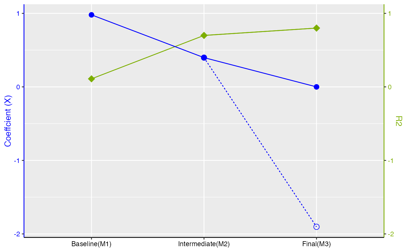
#> $Table
#> M1:X M2:X,Z M3(delta_exact):X,Z,CV M3(delta*):X,Z,CV
#> R2 0.1097571 0.7008711 8.006897e-01 0.8006897
#> coef_X 0.9798418 0.3980344 -1.114065e-16 -1.9033618
#> SE_X 0.1665047 0.0995086 8.775619e-02 0.2078153
#> std_coef_X 0.3266139 0.2297940 0.000000e+00 -0.6344539
#> t_X 5.8847685 4.0000000 -1.269500e-15 -9.1589120
#> coef_CV NA NA 2.049900e+00 4.8543646
#> SE_CV NA NA 1.702349e-01 0.4031330
#> t_CV NA NA 1.204159e+01 12.0415946
#>
#> $Figure
# using pkonfound for a 2x2 table
pkonfound(a = 35, b = 17, c = 17, d = 38)
#> Background Information:
#> This function calculates the number of cases that would have to be replaced
#> with no effect cases (RIR) to invalidate an inference made about the association
#> between the rows and columns in a 2x2 table.
#> One can also interpret this as switches from one cell to another, such as from
#> the treatment success cell to the treatment failure cell.
#>
#> Conclusion:
#> To invalidate the inference, you would need to replace 14 treatment success
#> cases for which the probability of failure in the control group applies (RIR = 14).
#> This is equivalent to transferring 9 cases from treatment success to treatment failure.
#> For the User-entered Table, we have an estimated odds ratio of 4.530, with p-value of 0.000:
#>
#> User-entered Table:
#> Fail Success
#> Control 35 17
#> Treatment 17 38
#>
#>
#> For the Transfer Table, we have an estimated odds ratio of 2.278, with p-value of 0.051:
#> Transfer Table:
#> Fail Success
#> Control 35 17
#> Treatment 26 29
#>
#> RIR:
#> RIR = 14
#> For other forms of output, run ?pkonfound and inspect the to_return argument
#> For models fit in R, consider use of konfound().
pkonfound(a = 35, b = 17, c = 17, d = 38, alpha = 0.01)
#> Background Information:
#> This function calculates the number of cases that would have to be replaced
#> with no effect cases (RIR) to invalidate an inference made about the association
#> between the rows and columns in a 2x2 table.
#> One can also interpret this as switches from one cell to another, such as from
#> the treatment success cell to the treatment failure cell.
#>
#> Conclusion:
#> To invalidate the inference, you would need to replace 9 treatment success
#> cases for which the probability of failure in the control group applies (RIR = 9).
#> This is equivalent to transferring 6 cases from treatment success to treatment failure.
#> For the User-entered Table, we have an estimated odds ratio of 4.530, with p-value of 0.000:
#>
#> User-entered Table:
#> Fail Success
#> Control 35 17
#> Treatment 17 38
#>
#>
#> For the Transfer Table, we have an estimated odds ratio of 2.835, with p-value of 0.011:
#> Transfer Table:
#> Fail Success
#> Control 35 17
#> Treatment 23 32
#>
#> RIR:
#> RIR = 9
#> For other forms of output, run ?pkonfound and inspect the to_return argument
#> For models fit in R, consider use of konfound().
pkonfound(a = 35, b = 17, c = 17, d = 38, alpha = 0.01, switch_trm = FALSE)
#> Background Information:
#> This function calculates the number of cases that would have to be replaced
#> with no effect cases (RIR) to invalidate an inference made about the association
#> between the rows and columns in a 2x2 table.
#> One can also interpret this as switches from one cell to another, such as from
#> the treatment success cell to the treatment failure cell.
#>
#> Conclusion:
#> To invalidate the inference, you would need to replace 19 control failure
#> cases for which the probability of failure in the control group applies (RIR = 19).
#> This is equivalent to transferring 6 cases from control failure to control success.
#> For the User-entered Table, we have an estimated odds ratio of 4.530, with p-value of 0.000:
#>
#> User-entered Table:
#> Fail Success
#> Control 35 17
#> Treatment 17 38
#>
#>
#> For the Transfer Table, we have an estimated odds ratio of 2.790, with p-value of 0.012:
#> Transfer Table:
#> Fail Success
#> Control 29 23
#> Treatment 17 38
#>
#> RIR:
#> RIR = 19
#> For other forms of output, run ?pkonfound and inspect the to_return argument
#> For models fit in R, consider use of konfound().
pkonfound(a = 35, b = 17, c = 17, d = 38, test = "chisq")
#> Background Information:
#> This function calculates the number of cases that would have to be replaced
#> with no effect cases (RIR) to invalidate an inference made about the association
#> between the rows and columns in a 2x2 table.
#> One can also interpret this as switches from one cell to another, such as from
#> the treatment success cell to the treatment failure cell.
#>
#> Conclusion:
#> To invalidate the inference, you would need to replace 15 treatment success
#> cases for which the probability of failure in the control group applies (RIR = 15).
#> This is equivalent to transferring 10 cases from treatment success to treatment failure.
#> For the User-entered Table, we have a Pearson's chi square of 14.176, with p-value of 0.000:
#>
#> User-entered Table:
#> Fail Success
#> Control 35 17
#> Treatment 17 38
#>
#>
#> For the Transfer Table, we have a Pearson's chi square of 3.640, with p-value of 0.056:
#> Transfer Table:
#> Fail Success
#> Control 35 17
#> Treatment 27 28
#>
#> RIR:
#> RIR = 15
#> For other forms of output, run ?pkonfound and inspect the to_return argument
#> For models fit in R, consider use of konfound().
# use pkonfound to calculate delta* and delta_exact
pkonfound(est_eff = .4, std_err = .1, n_obs = 290, sdx = 2, sdy = 6, R2 = .7, eff_thr = 0, FR2max = .8, index = "COP", to_return = "raw_output")
#> $`delta*`
#> [1] 3.668243
#>
#> $`delta*restricted`
#> [1] 4.085172
#>
#> $delta_exact
#> [1] 1.508536
#>
#> $delta_pctbias
#> [1] 143.1658
#>
#> $cor_oster
#> Y X Z CV
#> Y 1.0000000 0.3266139 0.8266047 0.2426367
#> X 0.3266139 1.0000000 0.2433792 0.8927742
#> Z 0.8266047 0.2433792 1.0000000 0.0000000
#> CV 0.2426367 0.8927742 0.0000000 1.0000000
#>
#> $cor_exact
#> Y X Z CV
#> Y 1.0000000 0.3266139 0.8266047 0.3416500
#> X 0.3266139 1.0000000 0.2433792 0.3671463
#> Z 0.8266047 0.2433792 1.0000000 0.0000000
#> CV 0.3416500 0.3671463 0.0000000 1.0000000
#>
#> $`var(Y)`
#> [1] 36
#>
#> $`var(X)`
#> [1] 4
#>
#> $`var(CV)`
#> [1] 1
#>
#> $Table
#> M1:X M2:X,Z M3(delta_exact):X,Z,CV M3(delta*):X,Z,CV
#> R2 0.1097571 0.7008711 8.006897e-01 0.8006897
#> coef_X 0.9798418 0.3980344 -1.114065e-16 -1.9033618
#> SE_X 0.1665047 0.0995086 8.775619e-02 0.2078153
#> std_coef_X 0.3266139 0.2297940 0.000000e+00 -0.6344539
#> t_X 5.8847685 4.0000000 -1.269500e-15 -9.1589120
#> coef_CV NA NA 2.049900e+00 4.8543646
#> SE_CV NA NA 1.702349e-01 0.4031330
#> t_CV NA NA 1.204159e+01 12.0415946
#>
#> $Figure
 #>
#> $`conditional RIR pi (fixed y)`
#> [1] 0.4842727
#>
#> $`conditional RIR (fixed y)`
#> [1] 140.4391
#>
#> $`conditional RIR pi (null)`
#> [1] 0.2818584
#>
#> $`conditional RIR (null)`
#> [1] 81.73894
#>
#> $`conditional RIR pi (rxyGz)`
#> [1] 0.4977821
#>
#> $`conditional RIR (rxyGz)`
#> [1] 144.3568
#>
# use pkonfound to calculate rxcv and rycv when preserving standard error
pkonfound(est_eff = .5, std_err = .056, n_obs = 6174, eff_thr = .1, sdx = 0.22, sdy = 1, R2 = .3, index = "PSE", to_return = "raw_output")
#> $`correlation between X and CV conditional on Z`
#> [1] 0.2479732
#>
#> $`correlation between Y and CV conditional on Z`
#> [1] 0.3721927
#>
#> $`correlation between X and CV`
#> [1] 0.2143186
#>
#> $`correlation between Y and CV`
#> [1] 0.313404
#>
#> $`covariance matrix`
#> Y X Z CV
#> Y 1.00000000 0.07777425 0.5394031 0.31340398
#> X 0.07777425 0.04840000 0.1106620 0.04715009
#> Z 0.53940306 0.11066202 1.0000000 0.00000000
#> CV 0.31340398 0.04715009 0.0000000 1.00000000
#>
#> $Table
#> M1:X M2:X,Z M3:X,Z,CV
#> R2 0.1251176 0.3001134 0.38959867
#> coef_X 1.6069060 0.5001620 0.09742753
#> SE_X 0.0541133 0.0560000 0.05398370
#> std_coef_X 0.3535193 0.1129410 0.02143406
#> t_X 29.6952137 8.9314651 1.80475837
#> coef_Z NA 0.4840541 0.52862153
#> SE_Z NA 0.0123200 0.01160045
#> t_Z NA 39.2901069 45.56905001
#> coef_CV NA NA 0.30881026
#> SE_CV NA NA 0.01026456
#> t_CV NA NA 30.08509668
#>
#>
#> $`conditional RIR pi (fixed y)`
#> [1] 0.4842727
#>
#> $`conditional RIR (fixed y)`
#> [1] 140.4391
#>
#> $`conditional RIR pi (null)`
#> [1] 0.2818584
#>
#> $`conditional RIR (null)`
#> [1] 81.73894
#>
#> $`conditional RIR pi (rxyGz)`
#> [1] 0.4977821
#>
#> $`conditional RIR (rxyGz)`
#> [1] 144.3568
#>
# use pkonfound to calculate rxcv and rycv when preserving standard error
pkonfound(est_eff = .5, std_err = .056, n_obs = 6174, eff_thr = .1, sdx = 0.22, sdy = 1, R2 = .3, index = "PSE", to_return = "raw_output")
#> $`correlation between X and CV conditional on Z`
#> [1] 0.2479732
#>
#> $`correlation between Y and CV conditional on Z`
#> [1] 0.3721927
#>
#> $`correlation between X and CV`
#> [1] 0.2143186
#>
#> $`correlation between Y and CV`
#> [1] 0.313404
#>
#> $`covariance matrix`
#> Y X Z CV
#> Y 1.00000000 0.07777425 0.5394031 0.31340398
#> X 0.07777425 0.04840000 0.1106620 0.04715009
#> Z 0.53940306 0.11066202 1.0000000 0.00000000
#> CV 0.31340398 0.04715009 0.0000000 1.00000000
#>
#> $Table
#> M1:X M2:X,Z M3:X,Z,CV
#> R2 0.1251176 0.3001134 0.38959867
#> coef_X 1.6069060 0.5001620 0.09742753
#> SE_X 0.0541133 0.0560000 0.05398370
#> std_coef_X 0.3535193 0.1129410 0.02143406
#> t_X 29.6952137 8.9314651 1.80475837
#> coef_Z NA 0.4840541 0.52862153
#> SE_Z NA 0.0123200 0.01160045
#> t_Z NA 39.2901069 45.56905001
#> coef_CV NA NA 0.30881026
#> SE_CV NA NA 0.01026456
#> t_CV NA NA 30.08509668
#>